Correlation and Regression
Emma Rand

Introduction
Aims
You will learn how to chose between correlation and regression as well as applying, interpreting and reporting them.
Learning Outcomes
By actively following the lecture and practical and carrying out the independent study the successful student will be able to:
- Explain the principles of correlation and of regression (MLO 1)
- Apply (appropriately), interpret and evaluate the legitimacy of, both in R (MLO 2, 3 and 4)
- Summarise and illustrate with appropriate R figures test results scientifically (MLO 3 and 4)
Philosophy
Workshops are not a test. It is expected that you often don’t know how to start, make a lot of mistakes and need help. Do not be put off and don’t let what you can not do interfere with what you can do. You will benefit from collaborating with others and/or discussing your results.
The lectures and the workshops are closely integrated and it is expected that you are familar with the lecture content before the workshop. You need not understand every detail as the workshop should build and consolidate your understanding. You may wish to refer to the slides as you work through the workshop schedule.
Exercises
Getting started
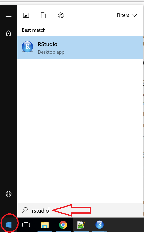
 Start RStudio from the Start menu.
 Make a new project with File | New Project and chose New directory and then New project. Be purposeful about where you create it by using the Browse button. I suggest using your 17C folder. Give the Project (directory) a name, perhaps “regress_correl”
Make a new folder ‘raw_data’ where you will later save data files.
Make a new folder ‘figures’ where you will later save your figures.
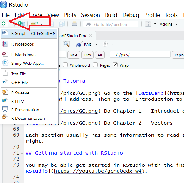
Make a new script file called analysis.R or similar to carry out the rest of the work.
You probably want to load the tidyverse with library(tidyverse).
Pearson’s Correlation
The data given in height.txt are the heights of eleven brother and sister pairs.
Save a copy of height.txt to your raw_data folder and import it.
Exploring
 What type of variables are ‘brother’ and ‘sister’? What are the implications for the test?
Do a quick plot of the data. We don’t have a causal relationship here so either varaible can go on the x-axis.

Remembering that one of the assumptions for parametric correlation is that any correlation should be linear, what do you conclude from the plot?
Applying, interpreting and reporting
We will do a parametric correlation in any case.
We can carry out a Pearson’s product moment correlation with:
##
##  Pearson's product-moment correlation
##
## data:  height$sister and height$brother
## t = 2.0157, df = 9, p-value = 0.07464
## alternative hypothesis: true correlation is not equal to 0
## 95 percent confidence interval:
##  -0.06336505  0.86739285
## sample estimates:
##       cor
## 0.5577091
What do you conclude from the test?
Illustrating
Create a better figure for our data using:
fig1 <- ggplot(height, aes(x = sister, y = brother)) +
  geom_point() +
  xlim(120, 180) +
  ylim(120, 190) +
  xlab("Heights of sister (cm)") +
  ylab("Heights of brother (cm)") +
  theme_classic()

fig1
Figure 1. Correlation in height between brothers and sisters.
Use ggsave() to save your figure to file. You can use what ever format you prefer (png, jpg, tiff eps). You may want to look up a previous week’s workshop.
Effect of sample size on correlation
Now we will explore the effect of sample size on the value of the correlation coefficient and its significance.
Create a dataset with twice the number of observation like this:
## 'data.frame':    22 obs. of  2 variables:
##  $ brother: num  180 173 168 170 178 ...
##  $ sister : num  175 163 165 160 165 ...
Each pair of values will apear twice.
Now repeat the correlation with height2
##
##  Pearson's product-moment correlation
##
## data:  height2$sister and height2$brother
## t = 3.0049, df = 20, p-value = 0.006999
## alternative hypothesis: true correlation is not equal to 0
## 95 percent confidence interval:
##  0.1779407 0.7928831
## sample estimates:
##       cor
## 0.5577091
What do you conclude? What does this tell you about the sensitivity of correlation to sample size?
Spearman’s rank Correlation
Since our brother-sister dataset is so small we might very reasonably have chosen to do a non-parametric correlation. This is very easy to do.
We just need to change the method:
##
##  Spearman's rank correlation rho
##
## data:  height$sister and height$brother
## S = 109.74, p-value = 0.1163
## alternative hypothesis: true rho is not equal to 0
## sample estimates:
##       rho
## 0.5011722
What do you conclude?
Linear Regression
The data in plant.xlsx is a set of observations of plant growth over two months. The researchers planted the seeds and harvested, dried and weighed a plant each day from day 10 so all the data points are independent of each other. There’s a good package for reading in Excel files, readxl. It is one of the tidyverse packages and will be installed when you install tidyverse but it is not one of the core packages that get loaded with library(tidyverse) therefore we need to library it. I recommend putting all your library statements together at the top of the file.
Save a copy of plant.xlsx to your raw_data folder and import it.
Excel workbooks can have multiple sheets. You can list the sheets in the workbook using excel_sheets()
What sheets are there in plant.xlsx?
## [1] "Sheet1" "plant" "Sheet2" "Sheet3" To read read the data in we use the read_excel() function
By default, the read_excel() function will read the first sheet in the workbook but the sheet option allows us to specify a particular sheet.
What type of variables do you have? Which is the response and which is the explanatory? What is the null hypothesis?
Exploring
Do a quick plot of the data (as shown) 
What are the assumptions of linear regression? Do these seem to be met?
Applying, interpreting and reporting
We now carry out a regression assigning the result of the lm() procedure to a variable and examining it with summary().
##
## Call:
## lm(formula = mass ~ day, data = plant)
##
## Residuals:
##     Min      1Q  Median      3Q     Max
## -32.810 -11.253  -0.408   9.075  48.869
##
## Coefficients:
##             Estimate Std. Error t value Pr(>|t|)
## (Intercept)  -8.6834     6.4729  -1.342    0.186
## day           1.6026     0.1705   9.401  1.5e-12 ***
## ---
## Signif. codes:  0 '***' 0.001 '**' 0.01 '*' 0.05 '.' 0.1 ' ' 1
##
## Residual standard error: 17.92 on 49 degrees of freedom
## Multiple R-squared:  0.6433, Adjusted R-squared:  0.636
## F-statistic: 88.37 on 1 and 49 DF,  p-value: 1.503e-12
The Estimates in the Coefficients table give the intercept (first line) and the slope (second line) of the best fitting straight line. The p-values in the same table are tests of whether that coefficient is different from zero.
The F value and p-value in the last line are a test of whether the model as a whole explains a significant amount of variation in the dependent variable. For a single linear regression this is exactly equivalent to the test of the slope against zero.
What is the equation of the line? What do you conclude from the analysis?
Does the line go through (0,0)?
What percentage of variation is explained by the line?
Checking selection
Check the assumptions of the test by looking at the distribution of the ‘residuals’.
Illustrating
We want a figure with the points and a best fitting straight line.
Create a figure with using both geom_point() and geom_smooth()
ggplot(plant, aes(x = day, y = mass)) +
  geom_point() +
  geom_smooth(method = lm, se = FALSE, colour = "black") +
  ylab("Mass (g)") +
  ylim(0, 120) +
  xlim(0, 65) +
  xlab("Day") +
  theme_classic()
Figure 2. The relationship between day since planting and mass.
Can you workout how to add the equation of the line to the figure?
Save your figure to your ‘figures’ folder.
Close your project, locate the folder in Windows Explorer and zip it by doing: Right click, Send to | Compressed (zipped) folder. Then email it to your neighbour and check they can open your unzipped project and have all the code work.
Independent study
Analyses
Decide how to analyse the following data sets. In each, use an RStudio project with logical directory structure. Organise and comment your code well and include your reasoning and decisions. Write your conclusions as comments in a form suitable for including in a report. Create and save an appropriate figure.
Effect of anxiety status and sporting performance
The data in sprint.txt are from an investigation of the effect of anxiety status and sporting performance. A group of 40 100m sprinters undertook a psychometric test to measure their anxiety shortly before competing. The data are their anxiety scores and the 100m times achieved. What you do conclude from these data?
Juvenile hormone in stag beetles
The concentration of juvenile hormone in stag beetles is known to influence mandible growth. Groups of stag beetles were injected with different concentrations of juvenile hormone (arbitrary units) and their average mandible size (mm) determined. The experimenters planned to analyse their data with regression. The data are in stag.txt
The Code files
These contain answers and code even though they do not appear on the webpage itself.
Rmd file The Rmd file is the file I use to compile the practical. Rmd stands for R markdown allow R code and ordinary text to be inter weaved to produce well-formatted reports including webpages.
Plain script file This is plain script (.R) version of the practical
Script example
This is an example of a well formatted analysis script for one of the independent study problems.
Objectives from previous sessions
Introduction to module and RStudio
- to explain why we need statistical tests and the logic of hypothesis testing (MLO 1)
- use the R command line as a calculator and to assign variables (MLO 3)
- create and use the basic data types in R (MLO 3)
- find their way around the RStudio windows (MLO 3)
- create, use and save a script file to run r commands (MLO 3)
- search and understand manual pages (MLO 3)
Testing, Data types and reading in data
- to able to explain what response and explanatory variables are, distinguish between data types and describe how these impact choice of test (MLO 1 and 2)
- demonstrate the process of hypothesis testing with an example and evaluate potential inferences (MLO 1 and 2)
- read in data in to RStudio, create simple summaries and plots using manual pages where necessary (MLO 3)
- create neat reports in Word which include text and figures (MLO 4)
Goodness of Fit and Contingency chi-squared tests
- recognise when to use chi-squared Goodness of Fit and Contingency tests (MLO 2)
- be able to carry out, interpret and report scientifically both types of test by hand and in R (MLO 3 and 4)
Calculating summary statistics, probabilities and confidence intervals
- Explain the properties of ‘normal distributions’ and their use in statistics (MLO 1 and 2)
- Define, select and calculate with R probabilities, quantiles and confidence intervals (MLO 3 and 4)
- Explain dependent and independent samples (MLO 2)
- Select, appropriately, t-tests and their non-parametric equivalents (MLO 2)
- Apply, interpret and evaluate the legitimacy of the tests in R (MLO 3 and 4)
- Summarise and illustrate with appropriate R figures test results scientifically (MLO 3 and 4)
One-way ANOVA and Kruskal-Wallis
- Explain the rationale behind ANOVA and complete a partially filled ANOVA table (MLO 1 and 2)
- Apply (appropriately), interpret and evaluate the legitimacy of, one-way ANOVA and Kruskal-Wallis including post-hoc tests in R (MLO 2, 3 and 4)
- Summarise and illustrate with appropriate R figures test results scientifically (MLO 3 and 4)
- Explain the rationale behind ANOVA and complete a partially filled ANOVA table (MLO 1 and 4)
- Read in data formatted for other statistical packages (MLO 3)
- Apply (appropriately), interpret and evaluate the legitimacy of, two-way ANOVA in R (MLO 2, 3 and 4)
- Explain the meaning of a significant interaction (MLO 4)
- Summarise and illustrate with appropriate figures test results scientifically (MLO 3 and 4)
- Use RStudio projects (MLO 4)
